내 풀이 github LINK: https://github.com/qkrtmdtj04/CS231n-Assignment
GitHub - qkrtmdtj04/CS231n-Assignment
Contribute to qkrtmdtj04/CS231n-Assignment development by creating an account on GitHub.
github.com
Two-Layer Neural Network의 한계 (Recap)
Assignment 1에서 구현한 Two-Layer Net은 입력층 → Hidden Layer → 출력층, 딱 두 개의 층으로 이루어진 구조였다. 수식으로 표현하면 아래와 같다.

이 구조는 선형 분류기보다 훨씬 강력하지만, 층이 고정되어 있다는 근본적인 한계가 있다. 현실의 복잡한 문제일수록 더 깊은 네트워크가 필요한데, 두 층짜리 코드를 그대로 쓰면 층을 추가할 때마다 코드를 통째로 다시 짜야한다.
Multi-Layer Network:
Assignment 2의 핵심 목표는 층의 개수(L)를 자유롭게 조절할 수 있는 범용 Fully Connected Network를 구현하는 것이다.
과제에서 요구하는 구조는 아래와 같다. (여담:batch, layer, dropout은 Q2,3 내용이며 개념은 다음 블로그에 서술할 예정이며, 이번 과제 코드에서는 추가되어 있다.)
{affine - [batch/layer norm] - relu - [dropout]} x (L - 1) - affine - softmax마지막 층 직전까지는 Affine + ReLU 블록을 L-1번 반복하고, 마지막 층은 활성화 함수 없이 Affine만 적용한 뒤 Loss를 계산한다. 이렇게 하면 num_layers=2로 설정하면 Assignment 1의 TwoLayerNet과 완전히 동일한 구조가 된다.
Update Rules:
지금까지는 가장 기본적인 SGD를 사용했다. SGD는 단순히 기울기 방향으로 일정 크기만큼 이동하는 방식인데, 깊은 네트워크일수록 Loss surface가 복잡해져 SGD만으로는 느리고 불안정한 경우가 많다.
문제를 구체적으로 보면, Loss surface는 대부분 안장점(Saddle Point)이나 좁고 긴 골짜기 형태를 띠는데 SGD는 이런 지형에서 비효율적으로 진동하거나 아예 멈춰버린다. 이를 해결하기 위해 더 영리하게 가중치를 업데이트하는 방법들이 등장했다.
크게 두 가지 방향의 접근법이 있다.
- 기울기의 방향에 관성을 주자 → SGD + Momentum
- 파라미터별로 학습률을 적응적으로 조정하자 → AdaGrad, RMSProp
- 둘 다 하자 → Adam
1. SGD + Momentum
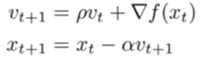
공이 경사면을 굴러 내려오는 것을 상상하면 쉽다. SGD가 매 스텝마다 현재 기울기만 보고 이동했다면, Momentum은 이전에 이동하던 속도(velocity)를 기억해 그 방향을 유지하려 한다. 덕분에 좁고 긴 골짜기에서 진동이 줄어들고, 안장점에서도 관성으로 빠져나올 수 있다.
2. RMSProp & AdaGrad

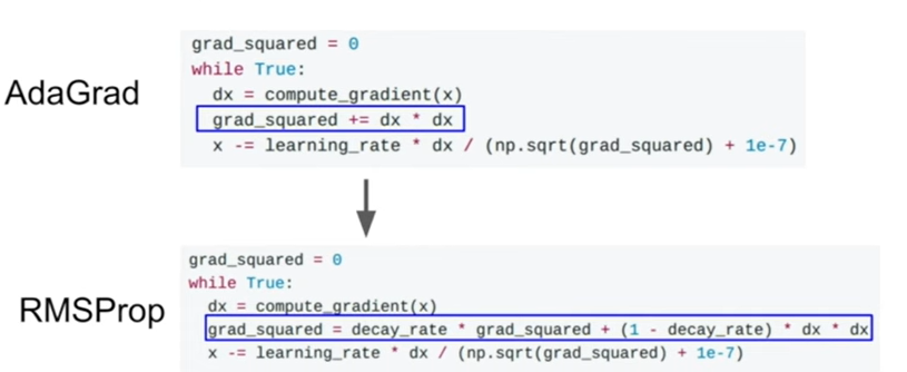
SGD+Momentum이 기울기의 방향에 집중했다면, 이 계열은 기울기의 크기를 파라미터별로 다르게 조정한다. 기울기가 크게 변한 방향은 학습률을 줄이고, 완만하게 변한 방향은 학습률을 키우는 방식이다.
AdaGrad는 cache += dw**2로 기울기 제곱을 무한정 누적하기 때문에 학습이 길어질수록 분모가 너무 커져 업데이트가 사실상 멈춰버리는 문제가 있다. RMSProp은 이를 해결하기 위해 단순 누적 대신 지수 이동평균을 사용해 오래된 기울기 정보는 자연스럽게 잊히도록 개선했다.
3. Adam
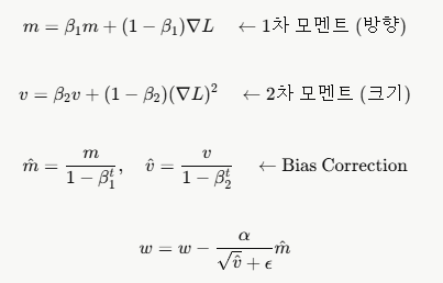
Adam은 Momentum(방향)과 RMSProp(크기)을 결합한 방식이다. 여기서 한 가지 추가된 핵심이 Bias Correction인데, 학습 초기에 m과 v가 모두 0으로 초기화되어 있어 초반 업데이트가 0 쪽으로 편향되는 문제를 1 - β^t로 나눠 보정한다. 현재 딥러닝 실무에서 가장 널리 쓰이는 옵티마이저이며, 별다른 이유가 없다면 Adam부터 시작하는 것이 일반적이다.
Q1 Multi-Layer Network 풀이
Q1-1 Multi-Layer Network init
- 층의 개수가 가변적이므로 반복문으로 각 층의 W와 b를 동적으로 초기화한다. Normalization을 사용할 경우 추가로 scale 파라미터 gamma(1로 초기화)와 shift 파라미터 beta(0으로 초기화)도 함께 저장한다.
- temp_dim을 이전 층의 출력 크기로 계속 갱신하면서 다음 층의 W shape을 결정하는 것이 포인트다. 마지막 층은 반복문 바깥에서 따로 처리한다.
def __init__(
        self,
        hidden_dims,
        input_dim=3 * 32 * 32,
        num_classes=10,
        dropout_keep_ratio=1,
        normalization=None,
        reg=0.0,
        weight_scale=1e-2,
        dtype=np.float32,
        seed=None,
    ):
        """Initialize a new FullyConnectedNet.

        Inputs:
        - hidden_dims: A list of integers giving the size of each hidden layer.
        - input_dim: An integer giving the size of the input.
        - num_classes: An integer giving the number of classes to classify.
        - dropout_keep_ratio: Scalar between 0 and 1 giving dropout strength.
            If dropout_keep_ratio=1 then the network should not use dropout at all.
        - normalization: What type of normalization the network should use. Valid values
            are "batchnorm", "layernorm", or None for no normalization (the default).
        - reg: Scalar giving L2 regularization strength.
        - weight_scale: Scalar giving the standard deviation for random
            initialization of the weights.
        - dtype: A numpy datatype object; all computations will be performed using
            this datatype. float32 is faster but less accurate, so you should use
            float64 for numeric gradient checking.
        - seed: If not None, then pass this random seed to the dropout layers.
            This will make the dropout layers deteriminstic so we can gradient check the model.
        """
        self.normalization = normalization
        self.use_dropout = dropout_keep_ratio != 1
        self.reg = reg
        self.num_layers = 1 + len(hidden_dims)
        self.dtype = dtype
        self.params = {}

        # *****START OF YOUR CODE (DO NOT DELETE/MODIFY THIS LINE)*****

        temp_dim = input_dim
        for layer in range(self.num_layers - 1): # affine - [batch/layer norm] - relu - [dropout]
            if normalization == 'batchnorm' or normalization == 'layernorm':
                self.params[f'W{layer+1}'] = np.random.randn(temp_dim, hidden_dims[layer]) * weight_scale
                self.params[f'b{layer+1}'] = np.zeros(hidden_dims[layer])
                self.params[f'gamma{layer+1}'] = np.ones(hidden_dims[layer])
                self.params[f'beta{layer+1}'] = np.zeros(hidden_dims[layer])
                temp_dim = hidden_dims[layer]

            else:
                self.params[f'W{layer+1}'] = np.random.randn(temp_dim, hidden_dims[layer]) * weight_scale
                self.params[f'b{layer+1}'] = np.zeros(hidden_dims[layer])
                temp_dim = hidden_dims[layer]

        # affine - softmax

        self.params[f'W{self.num_layers}'] = np.random.randn(temp_dim, num_classes) * weight_scale
        self.params[f'b{self.num_layers}'] = np.zeros(num_classes)

        # *****END OF YOUR CODE (DO NOT DELETE/MODIFY THIS LINE)*****
Q1-2. Forward Pass
- 각 층을 통과할 때마다 cache 딕셔너리에 키를 층 번호로 구분해 저장해 두는 것이 핵심이다. 나중에 역전 파할 때 같은 키로 꺼내 쓴다. Normalization과 Dropout은 self.normalization, self.use_dropout 플래그로 분기 처리해 선택적으로 적용한다.
Forward 과정에서는 각 층의 출력 shape가 다음 층 입력 shape로 그대로 전달된다.
(N, D)
 -> affine
(N, H1)
 -> relu
(N, H1)
 -> affine
(N, H2)
 ...
 -> affine
(N, C)
# *****START OF YOUR CODE (DO NOT DELETE/MODIFY THIS LINE)*****
#{affine - [batch/layer norm] - relu - [dropout]} x (L - 1) - affine - softmax
cache = {}
out=X
for layer in range(self.num_layers - 1):
if self.normalization == 'batchnorm':
out,cache[f"affine{layer}"] = affine_forward(out,self.params[f"W{layer+1}"],self.params[f"b{layer+1}"])
out,cache[f'batch{layer}'] = batchnorm_forward(out,self.params[f"gamma{layer+1}"],self.params[f"beta{layer+1}"],self.bn_params[layer])
out,cache[f"relu{layer}"] = relu_forward(out)
elif self.normalization == 'layernorm':
out,cache[f"affine{layer}"] = affine_forward(out,self.params[f"W{layer+1}"],self.params[f"b{layer+1}"])
out,cache[f'batch{layer}'] = layernorm_forward(out,self.params[f"gamma{layer+1}"],self.params[f"beta{layer+1}"],self.bn_params[layer])
out,cache[f"relu{layer}"] = relu_forward(out)
else:
out,cache[f"affine{layer}"] = affine_forward(out,self.params[f"W{layer+1}"],self.params[f"b{layer+1}"])
out,cache[f"relu{layer}"] = relu_forward(out)
if self.use_dropout:
out,cache[f"dropout{layer}"] = dropout_forward(out,self.dropout_param)
scores,cache[f"affine{self.num_layers}"] = affine_forward(out,self.params[f"W{self.num_layers}"],self.params[f"b{self.num_layers}"])
# *****END OF YOUR CODE (DO NOT DELETE/MODIFY THIS LINE)*****
Q1-3. Backward Pass
Forward의 정반대 순서로 진행한다. 주의할 점이 두 가지 있다.
- Dropout → ReLU → Norm → Affine 순서: Forward에서 쌓은 순서의 역순으로 정확히 풀어야 한다. Dropout을 먼저 역전파하고, 그다음 ReLU, 그다음 Normalization, 마지막으로 Affine 순이다.
- L2 Regularization: 매 층마다 0.5 * reg * W²를 Loss에 누적하고, dW에는 reg * W를 더해줘야 한다. 마지막 층은 반복문 바깥에서 따로 처리했기 때문에 반복문 안에서는 num_layers - 2부터 역순으로 돌린다.
        # *****START OF YOUR CODE (DO NOT DELETE/MODIFY THIS LINE)*****
        #print(cache.keys())
        loss,dx = softmax_loss(scores,y)
        reg = 0
        #print(cache.keys())

        dx, dw, db = affine_backward(dx,cache[f"affine{self.num_layers}"])
        grads[f'W{self.num_layers}'] = dw + self.reg * self.params[f'W{self.num_layers}']
        grads[f'b{self.num_layers}'] = db
        loss += 0.5 * self.reg * np.sum(self.params[f'W{self.num_layers}'] ** 2)


        for layer in range(self.num_layers - 2, -1, -1):
            if self.use_dropout:
                dx = dropout_backward(dx,cache[f"dropout{layer}"])
            dx = relu_backward(dx,cache[f"relu{layer}"])
            if self.normalization == 'batchnorm':
                dx, dgamma, dbeta = batchnorm_backward(dx,cache[f"batch{layer}"])
                grads[f'gamma{layer+1}'] = dgamma
                grads[f'beta{layer+1}'] = dbeta
            elif self.normalization == 'layernorm':
                dx, dgamma, dbeta = layernorm_backward(dx,cache[f"batch{layer}"])
                grads[f'gamma{layer+1}'] = dgamma
                grads[f'beta{layer+1}'] = dbeta
            dx, dw, db = affine_backward(dx,cache[f"affine{layer}"])
            grads[f'W{layer+1}'] = dw + self.reg * self.params[f'W{layer+1}']
            grads[f'b{layer+1}'] = db
            loss += np.sum(0.5 * self.reg * self.params[f'W{layer+1}'] * self.params[f'W{layer+1}'])

        # *****END OF YOUR CODE (DO NOT DELETE/MODIFY THIS LINE)*****
Q1-4. 신경망 층에 따른 과적합 문제
# TODO: Use a three-layer Net to overfit 50 training examples by
# tweaking just the learning rate and initialization scale.

num_train = 50
small_data = {
  "X_train": data["X_train"][:num_train],
  "y_train": data["y_train"][:num_train],
  "X_val": data["X_val"],
  "y_val": data["y_val"],
}

weight_scale = 1e-1   # Experiment with this!
learning_rate = 1e-3  # Experiment with this!
model = FullyConnectedNet(
    [100, 100],
    weight_scale=weight_scale,
    dtype=np.float64
)
solver = Solver(
    model,
    small_data,
    print_every=10,
    num_epochs=20,
    batch_size=25,
    update_rule="sgd",
    optim_config={"learning_rate": learning_rate},
)
solver.train()

plt.plot(solver.loss_history)
plt.title("Training loss history")
plt.xlabel("Iteration")
plt.ylabel("Training loss")
plt.grid(linestyle='--', linewidth=0.5)
plt.show()

# TODO: Use a five-layer Net to overfit 50 training examples by
# tweaking just the learning rate and initialization scale.

num_train = 50
small_data = {
  'X_train': data['X_train'][:num_train],
  'y_train': data['y_train'][:num_train],
  'X_val': data['X_val'],
  'y_val': data['y_val'],
}

learning_rate = 1e-1  # Experiment with this!
weight_scale = 1e-3   # Experiment with this!
model = FullyConnectedNet(
    [100, 100, 100, 100, 100],
    weight_scale=weight_scale,
    dtype=np.float64
)
solver = Solver(
    model,
    small_data,
    print_every=10,
    num_epochs=10,
    batch_size=25,
    update_rule='sgd',
    optim_config={'learning_rate': learning_rate},
)
solver.train()

plt.plot(solver.loss_history)
plt.title('Training loss history')
plt.xlabel('Iteration')
plt.ylabel('Training loss')
plt.grid(linestyle='--', linewidth=0.5)
plt.show()
Inline Question 1:
Did you notice anything about the comparative difficulty of training the three-layer network vs. training the five-layer network? In particular, based on your experience, which network seemed more sensitive to the initialization scale? Why do you think that is the case?
Answer:
3층은 표현력이 상대적으로 단순해 소규모 데이터를 빠르게 암기(과적합)한다. 반면 5층은 층이 깊어질수록 기울기가 역전 파 되는 경로가 길어지기 때문에, 초기화 스케일이 조금만 잘못돼도 기울기가 앞쪽 층까지 제대로 전달되지 않는다. 신호가 너무 크면 폭발(Exploding Gradient), 너무 작으면 소멸(Vanishing Gradient)해버리기 때문이다. 그래서 5층 네트워크가 초기화 스케일에 훨씬 더 민감하고, 같은 하이퍼파라미터로는 충분히 훈련되지 못한 것처럼 보이는 것이다. 이 문제를 근본적으로 해결하는 것이 바로 다음에 다룰 Batch Normalization이다.
Q1-5. Update Rules 구현
SGD + Momentum
def sgd_momentum(w, dw, config=None):
    if config is None:
        config = {}
    config.setdefault("learning_rate", 1e-2)
    config.setdefault("momentum", 0.9)
    v = config.get("velocity", np.zeros_like(w))

    v = config['momentum'] * v - config['learning_rate'] * dw
    next_w = w + v

    config["velocity"] = v
    return next_w, config
수식 그대로를 코드로 옮긴 것이라 간단하다. velocity를 config에서 꺼내 모멘텀 비율만큼 유지하면서 현재 기울기를 빼주고, 그 속도를 현재 가중치에 더해주면 끝이다. 주의할 점은 next_w = w + v에서 부호인데, v를 계산할 때 이미 -learning_rate * dw로 부호 처리를 했기 때문에 마지막엔 더하기로 마무리한다.
RMSProp
def rmsprop(w, dw, config=None):
    if config is None:
        config = {}
    config.setdefault("learning_rate", 1e-2)
    config.setdefault("decay_rate", 0.99)
    config.setdefault("epsilon", 1e-8)
    config.setdefault("cache", np.zeros_like(w))

    config['cache'] = config['decay_rate'] * config['cache'] + (1 - config['decay_rate']) * dw * dw
    next_w = w - (config['learning_rate'] * dw) / (np.sqrt(config['cache']) + config['epsilon'])

    return next_w, config
cache를 지수 이동평균으로 업데이트하는 것이 핵심이다. decay_rate(기본값 0.99)가 클수록 오래된 기울기 정보를 오래 기억하고, 작을수록 최근 기울기에 더 민감하게 반응한다. 분모에 epsilon을 더하는 것은 cache가 0에 가까울 때 나눗셈이 폭발하는 것을 방지하기 위한 안전장치다.
Adam
def adam(w, dw, config=None):
    if config is None:
        config = {}
    config.setdefault("learning_rate", 1e-3)
    config.setdefault("beta1", 0.9)
    config.setdefault("beta2", 0.999)
    config.setdefault("epsilon", 1e-8)
    config.setdefault("m", np.zeros_like(w))
    config.setdefault("v", np.zeros_like(w))
    config.setdefault("t", 0)

    config['t'] += 1

    config['m'] = config['beta1'] * config['m'] + (1 - config['beta1']) * dw
    mt = config['m'] / (1 - config['beta1'] ** config['t'])

    config['v'] = config['beta2'] * config['v'] + (1 - config['beta2']) * dw * dw
    vt = config['v'] / (1 - config['beta2'] ** config['t'])

    next_w = w - (config['learning_rate'] * mt) / (np.sqrt(vt) + config['epsilon'])

    return next_w, config
- 구현 순서가 중요하다. 주석에도 명시되어 있듯이 t를 먼저 증가시키고 나서 나머지 계산에 사용해야 한다. 그렇지 않으면 Bias Correction 값이 어긋나 결과가 달라진다.
코드를 단계별로 풀어보면 다음과 같다.
- t += 1: 스텝 카운터를 먼저 올린다.
- m 업데이트: 기울기의 1차 모멘트(방향)를 지수 이동평균으로 추적한다.
- mt: m을 1 - β1^t로 나눠 초기 편향을 보정한다.
- v 업데이트: 기울기 제곱의 2차 모멘트(크기)를 지수 이동평균으로 추적한다.
- vt: v를 1 - β2^t로 나눠 초기 편향을 보정한다.
- next_w: 보정된 mt와 vt를 이용해 가중치를 업데이트한다.
비교
# SGD vs SGD+Momentum 비교
for update_rule in ['sgd', 'sgd_momentum']:
    model = FullyConnectedNet([100, 100, 100, 100, 100], weight_scale=5e-2)
    solver = Solver(model, small_data,
        num_epochs=5, batch_size=100,
        update_rule=update_rule,
        optim_config={'learning_rate': 5e-3},
    )
    solvers[update_rule] = solver
    solver.train()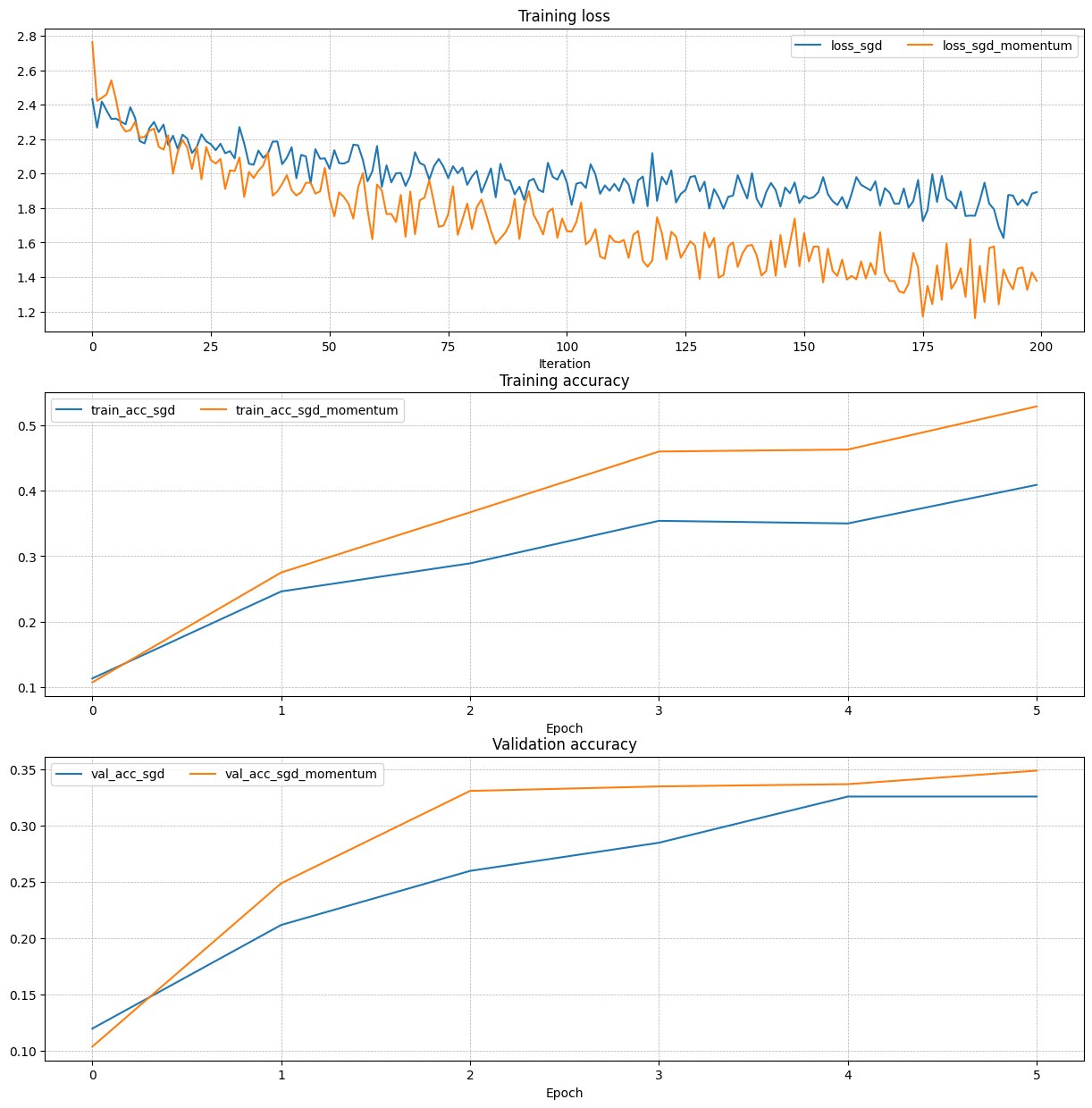
# RMSProp vs Adam 비교
learning_rates = {'rmsprop': 1e-4, 'adam': 1e-3}
for update_rule in ['adam', 'rmsprop']:
    model = FullyConnectedNet([100, 100, 100, 100, 100], weight_scale=5e-2)
    solver = Solver(model, small_data,
        num_epochs=5, batch_size=100,
        update_rule=update_rule,
        optim_config={'learning_rate': learning_rates[update_rule]},
    )
    solvers[update_rule] = solver
    solver.train()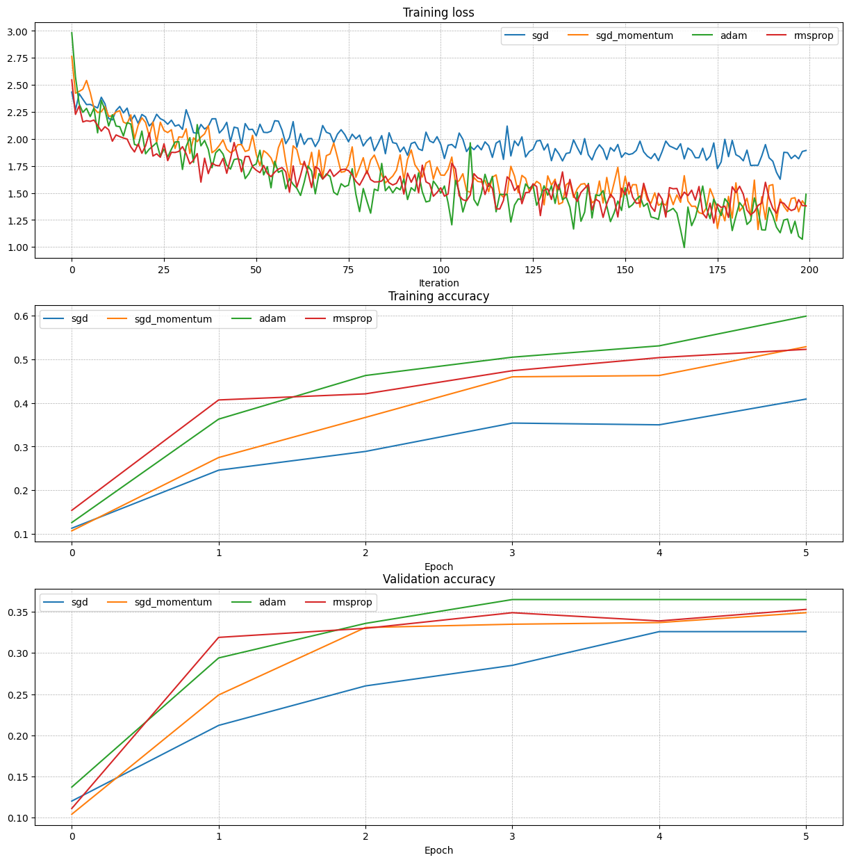
그래프를 보면 SGD+Momentum이 Vanilla SGD보다 훨씬 빠르게 수렴하고, Adam이 RMSProp보다 전반적으로 안정적인 것을 확인할 수 있다.
Inline Question 2:
AdaGrad, like Adam, is a per-parameter optimization method that uses the following update rule:
cache += dw**2w += - learning_rate * dw / (np.sqrt(cache) + eps)
John notices that when he was training a network with AdaGrad that the updates became very small, and that his network was learning slowly. Using your knowledge of the AdaGrad update rule, why do you think the updates would become very small? Would Adam have the same issue?
Answer:
[FILL THIS IN]
AdaGrad는 cache += dw**2로 기울기 제곱을 계속 누적만 하기 때문에 학습이 길어질수록 분모가 무한정 커진다. 분자는 그대로인데 분모만 커지니 업데이트 크기가 결국 0에 수렴해 버린다. Adam은 분자에 1차 모멘텀을 추가해 크기를 유지하고, 분모의 2차 모멘텀도 지수 이동평균으로 계산해 오래된 기울기는 자연스럽게 잊히도록 설계되어 있다. 덕분에 분자와 분모가 동시에 비슷한 비율로 움직여 업데이트가 죽지 않는다. 따라서 Adam은 같은 문제가 발생하지 않는다.
Q1-6. 최고 모델 탐색: 하이퍼파라미터 스윕
(Q2,3을 완료해야 할 수 있다.)
normalization = ['batchnorm', 'layernorm']
dropout_keep_ratio = [1, 0.75, 0.5, 0.25]
weight_scale = [5e-2, 1e-2]
learning_rates = {'rmsprop': 1e-4, 'adam': 1e-3}

for norm in normalization:
    for dropout in dropout_keep_ratio:
        for ws in weight_scale:
            model = FullyConnectedNet(
                [100, 100, 100, 100, 100],
                dropout_keep_ratio=dropout,
                normalization=norm,
                weight_scale=ws
            )
            for update_rule in ['adam', 'rmsprop']:
                solver = Solver(model, data,
                    num_epochs=20, batch_size=100,
                    update_rule=update_rule,
                    optim_config={'learning_rate': learning_rates[update_rule]},
                )
                solver.train()
Normalization 방식, Dropout 비율, Weight Scale, Optimizer를 모두 조합해 전수 탐색한다. 조합 수가 많아 시간이 꽤 걸리지만, 어떤 조합이 잘 되고 안 되는지 체계적으로 파악할 수 있다.
최종 결과
Validation set accuracy:  0.555
Test set accuracy:  0.55
Best validation accuracy achieved: 0.5580
목표인 50%를 넘어 55.5% 까지 달성했다. Batch Normalization + Adam 조합이 가장 안정적으로 높은 성능을 보였고, Dropout도 과적합 방지에 확실히 도움이 됐다.
마무리
이번 Q1에서 가장 인상 깊었던 것은 구조의 일반화와 Optimizer의 영향력 두 가지다. Assignment 1에서 층을 직접 손으로 이어 붙였던 것을 반복문 하나로 몇 층이든 자유롭게 쌓을 수 있게 바꿨고, 그 위에서 SGD부터 Adam까지 직접 구현하며 비교해 보니 옵티마이저 선택이 성능에 얼마나 큰 영향을 미치는지 체감할 수 있었다. 단순히 "Adam 쓰면 잘 된다"를 외우는 게 아니라, 왜 잘 되는지를 수식 단위로 이해하고 넘어가는 것이 결국 실력이 된다고 느꼈다.
'DeepLearning > CS231n' 카테고리의 다른 글
| CS231n Assignment 2: Q3: Dropout (0) | 2026.06.06 |
|---|---|
| CS231n Assignment 2: Q2: Batch Normalization (0) | 2026.05.30 |
| CS231n Assignment 1: Q4: Two-Layer Neural Network (0) | 2026.04.04 |
| CS231n Assignment 1: Q3 Implement a Softmax classifier (0) | 2026.03.08 |
| CS231n Assignment 1: Q2 Support Vector Machine (0) | 2026.03.07 |


