내 풀이 github LINK: https://github.com/qkrtmdtj04/CS231n-Assignment
GitHub - qkrtmdtj04/CS231n-Assignment
Contribute to qkrtmdtj04/CS231n-Assignment development by creating an account on GitHub.
github.com
Linear Classification의 한계 (Recap)
- 지금까지 배운 SVM이나 Softmax는 결국 하나의 선(Linear)으로 데이터를 분류하는 방식이었다. 하지만 실제 데이터는 복잡하게 얽혀 있어 선 하나로는 분류하기 어려운 경우가 많다.
- 이를 해결하기 위해 여러 개의 선을 겹치고, 그 사이에 '비선형성'을 추가한 것이 바로 Neural Network이다.
Two-Layer Neural Network
- 이름 그대로 층이 두 개다. 입력층(Input)에서 바로 결과로 가는 게 아니라, 중간에 Hidden Layer(은닉층)를 하나 거친다.
- 수식으로 표현하면 다음과 같다. 위는 선형함수, 아래는 Two-Layer Neural Network
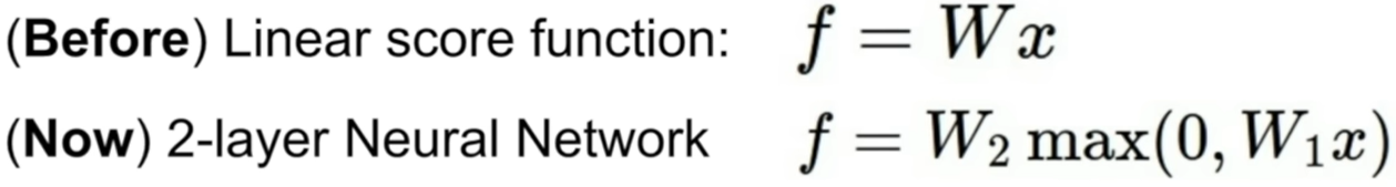
- W_1을 통해 특징을 추출하고, ReLU라는 활성화 함수를 거친 뒤, 다시 W_2를 곱해 최종 점수를 내는 방식이다.
1. 활성화 함수: ReLU (Rectified Linear Unit)
- 위 수식에서 max(0, score)에 해당한다.
- 0보다 작으면 0을 반환하고, 0보다 크면 그 값을 그대로 유지한다. 이 간단한 함수가 네트워크에 비선형성(Non-linearity)을 부여해 복잡한 패턴을 학습할 수 있게 만든다.
2. Backpropagation (역전파)
- NN에서 가장 중요한 개념이다. 층이 깊어질수록 Loss에 대한 각 가중치의 미분 값을 구하기가 복잡해지는데, 이를 Chain Rule(연쇄 법칙)을 이용해 뒤에서부터 앞으로 에러를 전달하며 계산하는 방식이다.
Q4 Two-Layer Neural Network:풀이
Q4-1 & Q4-2: Affine Layer (Fully Connected Layer)
- 가장 기본이 되는 선형 변환 층이다. 입력 데이터를 가중치와 내적 하고 편향(bias)을 더한다.
Forward Pass
입력 x를 2차원 행렬로 변환(Flatten)하여 연산하는 것이 포인트다.
def affine_forward(x, w, b):
    num_train = x.shape[0]
    # (N, D) @ (D, H) -> (N, H)
    out = np.dot(x.reshape(num_train, -1), w) + b
    cache = (x, w, b)
    return out, cache
Backward Pass
역전파 시에는 미분의 연쇄 법칙(Chain Rule)을 적용한다.
def affine_backward(dout, cache):
    x, w, b = cache
    # dx: dout @ w.T (입력 데이터 형태에 맞게 리셰이프)
    dx = np.dot(dout, w.T).reshape(x.shape)
    # dw: x.T @ dout
    dw = np.dot(x.reshape(x.shape[0], -1).T, dout)
    # db: dout의 열 방향 합
    db = np.sum(dout, axis=0)
    return dx, dw, db
Q4-3 & Q4-4: ReLU Layer
비선형성을 부여하는 활성화 함수 층이다.
- Forward: np.maximum(0, x)를 통해 음수 값을 0으로 차단한다.
- Backward: 입력 x가 0보다 컸던 지점은 기울기를 그대로 전달하고, 0 이하였던 지점은 기울기를 0으로 만든다.
- Backward: (dx = dout * (x >= 0))
Inline Question 1: Vanishing Gradient
- Q: 어떤 활성화 함수가 Gradient Flow를 차단(Zero gradient)하는 문제를 일으키는가?
- A: Sigmoid와 ReLU.
- Sigmoid: 입력값이 너무 크거나 작으면 기울기가 0에 수렴한다.
- ReLU: 입력값이 음수일 경우 기울기를 0으로 고정하기 때문에 'Dead ReLU' 문제가 발생할 수 있다.
Q4-5: TwoLayerNet 클래스 구현
1. 가중치 초기화 (init)
가중치는 Gaussian 분포로 아주 작게 초기화하고, Bias는 0으로 초기화한다.
self.params['W1'] = np.random.randn(input_dim, hidden_dim) * weight_scale
self.params['b1'] = np.zeros(hidden_dim)
self.params['W2'] = np.random.randn(hidden_dim, num_classes) * weight_scale
self.params['b2'] = np.zeros(num_classes)
2. Loss 및 Gradient 계산
    def loss(self, X, y=None):
        scores = None
        ############################################################################
        # TODO: Implement the forward pass for the two-layer net, computing the    #
        # class scores for X and storing them in the scores variable.              #
        ############################################################################
        # *****START OF YOUR CODE (DO NOT DELETE/MODIFY THIS LINE)*****

        layer1_out,layer1_cache = affine_forward(X,self.params['W1'],self.params['b1'])
        layer1_relu_out,layer1_relu_cache = relu_forward(layer1_out)
        layer2_out,layer2_cache = affine_forward(layer1_relu_out,self.params['W2'],self.params['b2'])
        scores = layer2_out

        # *****END OF YOUR CODE (DO NOT DELETE/MODIFY THIS LINE)*****
        ############################################################################
        #                             END OF YOUR CODE                             #
        ############################################################################

        # If y is None then we are in test mode so just return scores
        if y is None:
            return scores

        loss, grads = 0, {}
        ############################################################################
        # TODO: Implement the backward pass for the two-layer net. Store the loss  #
        # in the loss variable and gradients in the grads dictionary. Compute data #
        # loss using softmax, and make sure that grads[k] holds the gradients for  #
        # self.params[k]. Don't forget to add L2 regularization!                   #
        #                                                                          #
        # NOTE: To ensure that your implementation matches ours and you pass the   #
        # automated tests, make sure that your L2 regularization includes a factor #
        # of 0.5 to simplify the expression for the gradient.                      #
        ############################################################################
        # *****START OF YOUR CODE (DO NOT DELETE/MODIFY THIS LINE)*****

        loss,softmaxdx = softmax_loss(scores,y)

        layer1_reg = 0.5 * self.reg * self.params['W1'] * self.params['W1']
        layer2_reg = 0.5 * self.reg * self.params['W2'] * self.params['W2']
        loss += np.sum(layer1_reg) + np.sum(layer2_reg)

        layer2_dx, layer2_dW, layer2_db = affine_backward(softmaxdx,layer2_cache)
        layer2_dW += self.reg * self.params['W2']
        grads['W2'] = layer2_dW
        grads['b2'] = layer2_db

        relu_dx = relu_backward(layer2_dx,layer1_relu_cache)

        layer1_dx, layer1_dW, layer1_db = affine_backward(relu_dx,layer1_cache)
        layer1_dW += self.reg * self.params['W1']
        grads['W1'] = layer1_dW
        grads['b1'] = layer1_db


        # *****END OF YOUR CODE (DO NOT DELETE/MODIFY THIS LINE)*****
        ############################################################################
        #                             END OF YOUR CODE                             #
        ############################################################################

        return loss, grads
앞서 만든 모듈들을 조립하는 단계다.
- Forward: affine_forward → relu_forward → affine_forward 순으로 진행한다.
- Softmax: 최종 scores를 이용해 Loss와 초기 dout을 구한다.
- Backward: 역순으로 affine_backward → relu_backward → affine_backward를 호출하며 각 가중치의 기울기를 grads 딕셔너리에 저장한다. 이때 L2 Regularization 미분값(self.reg * W)을 더해주는 것을 잊으면 안 된다.
Q4-6: Solver를 통한 학습
직접 Optimizer를 짜는 대신, 제공된 Solver 클래스를 활용해 모델을 학습시킨다.
from functools import lru_cache
input_size = 32 * 32 * 3
hidden_size = 50
num_classes = 10
model = TwoLayerNet(input_size, hidden_size, num_classes)
solver = None

##############################################################################
# TODO: Use a Solver instance to train a TwoLayerNet that achieves about 36% #
# accuracy on the validation set.                                            #
##############################################################################
# *****START OF YOUR CODE (DO NOT DELETE/MODIFY THIS LINE)*****

solver = Solver(model, data,
    optim_config={
        'learning_rate': 1e-3,
    },
)
solver.train()
# *****END OF YOUR CODE (DO NOT DELETE/MODIFY THIS LINE)*****
##############################################################################
#                             END OF YOUR CODE                               #
##############################################################################
Q4-6 & Q4-7: Solver 사용 및 하이퍼파라미터 튜닝
직접 학습 루프를 짜는 대신 Solver 클래스를 활용해 최적의 모델을 찾는다.
best_model = None
best_acc = -1
results = {}
#################################################################################
# TODO: Tune hyperparameters using the validation set. Store your best trained #
# model in best_model. #
# #
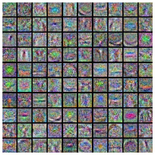
# To help debug your network, it may help to use visualizations similar to the #
# ones we used above; these visualizations will have significant qualitative #
# differences from the ones we saw above for the poorly tuned network. #
# #
# Tweaking hyperparameters by hand can be fun, but you might find it useful to #
# write code to sweep through possible combinations of hyperparameters #
# automatically like we did on thexs previous exercises. #
#################################################################################
# *****START OF YOUR CODE (DO NOT DELETE/MODIFY THIS LINE)*****
#model Hyperparameter
regs =[0.,0.05]
hidden_dims = [50,100]
#solver Hyperparameter
learning_rates = [1e-2,1e-3]
for reg in regs:
for hidden_dim in hidden_dims:
for lr in learning_rates:
model = TwoLayerNet(hidden_dim=hidden_dim,reg=reg)
solver = Solver(model,data,optim_config={'learning_rate':lr},verbose=False)
solver.train()
acc = solver.check_accuracy(data['X_val'],data['y_val'])
if acc > best_acc:
best_acc = acc
best_model = model
results[(lr,reg,hidden_dim)] = acc
for lr,reg,hd in sorted(results):
print('learning rates:',lr, 'regularization:',reg, 'hidden_dims:',hd, 'accuracy:', results[(lr,reg,hd)])
print('best accuracy is:', best_acc)
# *****END OF YOUR CODE (DO NOT DELETE/MODIFY THIS LINE)*****
################################################################################
# END OF YOUR CODE #
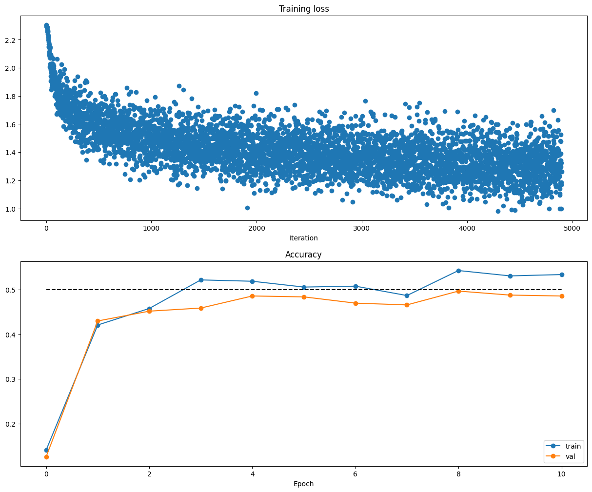
################################################################################# 하이퍼파라미터 스윕 결과
learning rates: 0.001 regularization: 0.0 hidden_dims: 100 accuracy: 0.506
learning rates: 0.01 regularization: 0.05 hidden_dims: 100 accuracy: 0.126
코드 해설
- 학습 결과: learning_rate가 0.01일 때는 정확도가 급격히 떨어지는 것을 볼 수 있다. 이는 보폭(Step size)이 너무 커서 최적점을 지나쳐 발산했기 때문이다.
- Best Model: 최종적으로 50.6%라는 정확도를 얻었고 선형 분류기가 30%대에 머물렀던 것에 비하면 엄청난 성능 향상이다.
Inline Question 2: Overfitting 방지
Q: 훈련 정확도와 테스트 정확도의 격차(Gap)를 줄이는 방법은? A: 1번(Large dataset)과 3번(Regularization strength 증가).
해설
1번은 데이터를 늘리는 것은 과적합되는것을 방지해 주며 특징 값들을 좀 더 많이 알아낼 수 있기 때문이다.
3번(정규화 강도 증가) 정규화는 모델이 훈련 데이터의 노이즈까지 학습하지 못하도록 '규제'를 거는 것이기 때문에, 훈련/테스트 정확도 사이의 간격을 줄이는(Generalization) 대표적인 방법이다. 반면 2번(Hidden units 추가)은 모델을 더 복잡하게 만들어 오히려 과적합을 심화시킬 수 있다.
'DeepLearning > CS231n' 카테고리의 다른 글
| CS231n Assignment 2: Q2: Batch Normalization (0) | 2026.05.30 |
|---|---|
| CS231n Assignment 2: Q1: Multi-Layer Fully Connected Neural Networks (0) | 2026.05.21 |
| CS231n Assignment 1: Q3 Implement a Softmax classifier (0) | 2026.03.08 |
| CS231n Assignment 1: Q2 Support Vector Machine (0) | 2026.03.07 |
| CS231n Assignment 1: Q1 k-NN (0) | 2026.03.02 |


